
F.21. Hydra Optimized Row Columnar (ORC)#
F.21. Hydra Optimized Row Columnar (ORC) #
- F.21.1. About Hydra Columnar
- F.21.2. Intro
- F.21.3. Columnar Installation
- F.21.4. Basic principles and questions
- F.21.5. Columnar Usage
- F.21.6. Performance Microbenchmarks
- F.21.7. Row vs Column Tables
- F.21.8. Updates and Deletes
- F.21.9. Optimizing Query Performance
- F.21.10. Materialized Views
- F.21.11. Vectorized Execution
- F.21.12. Query Parallelization
- F.21.13. Common recomendations
- F.21.14. Working with Time Series Data
F.21.2. Intro #
In traditional analytical (OLAP) systems, data size and volume tend to increase over time, potentially leading to various performance challenges. Columnar storage offers considerable advantages, especially in scenarios where database management systems (DBMSs) are employed for analytical tasks that predominantly involve batch data loading.
Columnar storage allows for substantial table compression, greatly reducing resource usage while maintaining high performance. This is achievable without resorting to distributed MPP (Massive Parallel Processing) DBMS systems. The inherent structure of ORC in Columnar storage facilitates efficient disk reads and offers superior data compression, enhancing overall performance.
Note
While the Columnar storage approach doesn't entirely supplant distributed MPP (Massive Parallel Processing) DBMSs in analytics, it can eliminate the need for them in certain situations. The decision to transition to an MPP DBMS depends on specific data volumes and workload demands. Although this threshold varies, it is generally in the realm of tens of terabytes.
F.21.3. Columnar Installation #
The Columnar storage method is set as an extension. To add Columnar to your local Tantor SE database, connect with psql and run:
CREATE EXTENSION pg_columnar;
F.21.4. Basic principles and questions #
F.21.4.1. Columnar basic principles #
Tantor SE standard heap data storage method
works well for an OLTP workload:
Support
UPDATE/DELETEoperations,Efficient single-tuple lookups
Columnar tables are best suited for analytic or data warehouse workloads, where the following benefits will be useful compared to the heap method:
Compression
Doesn't read unnecessary columns
Efficient VACUUM.
F.21.4.2. Why is Hydra Columnar so fast? #
There are a number of reasons for this:
Column-level caching
Tuning Tantor SE
F.21.4.3. What operations is Hydra Columnar meant for? #
Aggregates (COUNT, SUM, AVG), WHERE clauses, bulk INSERTs, UPDATE, DELETE and others.
F.21.4.4. What is columnar not meant for? #
Frequent large updates, small transactions.
Hydra Columnar supports both row and columnar tables, and any storage format has tradeoffs.
Columnar is not best for:
Datasets that have frequent large updates. While updates on Hydra Columnar are supported, they are slower than on heap tables.
Small transactions, particularly when the query needs to return very quickly, since each columnar transaction is quite a bit slower than a heap transaction.
Queries where traditional indexes provide high cardinality (i.e. are very effective), e.g. “needle in a haystack” problems, like “find by ID.” For this reason, reference join tables are best stored using a heap table.
Very large single table datasets may need special care to perform well, like using table partitioning. We plan to improve this further in the future. If you are tackling a “big data” problem, reach out to us for help!
Use cases where high concurrency is needed. Analytical queries on Hydra Columnar make extensive use of parallelization, and thus consume large amounts of resources, limiting the ability to run queries concurrently.
Where columnar falls short, traditional heap tables can often help. On Hydra Columnar you can mix both!
F.21.4.5. What Tantor SE features are unsupported on columnar? #
Columnar tables do not support logical replication.
Foreign keys are not supported.
F.21.4.6. How does Hydra Columnar handle complex queries? #
Try Incremental Materialized views.
Materialized views are precomputed database tables that store the results of a query. Hydra Columnar offers automatic updates to materialized views based on changes in the underlying base tables. This approach eliminates the need to recalculate the entire view, resulting in improved query performance and without time-consuming recomputation.
F.21.5. Columnar Usage #
F.21.5.1. Should I use a row or columnar table? #
Please see our section about when to use row and columnar tables.
F.21.5.2. Enabling Columnar #
Create need to have columnar enabled by running the query below as superuser:
CREATE EXTENSION IF NOT EXISTS pg_columnar;
Once installed, you will not need superuser to utilize columnar tables.
F.21.5.3. Using a columnar table #
Creating a columnar table, specifying the
USING columnar option:
CREATE TABLE my_columnar_table
(
    id INT,
    i1 INT,
    i2 INT8,
    n NUMERIC,
    t TEXT
) USING columnar;
Insert the data into the table and read it as usual (subject to the restrictions listed above).
To view internal statistics for a table, use
VACUUM VERBOSE. Note that
VACUUM (without FULL) is
much faster on a columnar table because it only scans the
metadata and not the actual data.
Set table options using columnar.alter_columnar_table_set:
SELECT columnar.alter_columnar_table_set(
  'my_columnar_table',
  compression => 'none',
  stripe_row_limit => 10000
);
For tables following options are available:
columnar.compression:
['none'|'pglz'|'zstd'|'lz4'|'lz4hc']- set compression type for newly inserted data. Existing data will not be recompressed/decompressed. The default value is'zstd'(if support was specified when compiling).columnar.compression_level:
<integer>- sets the compression level. Valid values are1to19. If the compression method does not support the selected level, the closest level will be selected instead. The default value is3.columnar.stripe_row_limit:
<integer>- the maximum number of rows in a stripe for newly inserted data. Existing data stripes will not be modified and may contain more rows than this maximum value. Valid values are1000to100000000. The default value is150000.columnar.chunk_group_row_limit:
<integer>- maximum number of rows in a chunk for newly inserted data. Existing data chunks will not be modified and may have more rows than this maximum value. Valid values are1000to100000000. The default value is10000.
You can view the options of all tables using:
SELECT * from columnar.options;
Or a specific table:
SELECT * FROM columnar.options
WHERE regclass = 'my_columnar_table'::regclass;
You can reset one or more table options to their default (or current values using SET)
using columnar.alter_columnar_table_reset:
SELECT columnar.alter_columnar_table_reset(
  'my_columnar_table',
  chunk_group_row_limit => true
);
Set general columnar options using SET:
SET columnar.compression TO 'none';
SET columnar.enable_parallel_execution TO false;
SET columnar.compression TO default;
columnar.enable_parallel_execution:
<boolean>- enables parallel execution. The default value istrue.columnar.min_parallel_processes:
<integer>- minimum number of parallel processes. Valid values are1to32. The default value is8.columnar.enable_vectorization:
<boolean>- enables vectorized execution. The default value istrue.columnar.enable_dml:
<boolean>- enables DML. The default value istrue.columnar.enable_column_cache:
<boolean>- enables column based caching. The default value isfalse.columnar.column_cache_size:
<integer>- size of the column based cache in megabytes. Valid values are20to20000. The default value is200. You can also specify a value with a unit of measurement, for example,'300MB'or'4GB'.columnar.enable_columnar_index_scan:
<boolean>- enables custom columnar index scan. The default value isfalse.columnar.enable_custom_scan:
<boolean>- enables the use of a custom scan to push projections and quals into the storage layer. The default value istrue.columnar.enable_qual_pushdown:
<boolean>- enables qual pushdown into columnar. This has no effect unlesscolumnar.enable_custom_scanistrue. The default value istrue.columnar.qual_pushdown_correlation_threshold:
<real>- correlation threshold to attempt to push a qual referencing the given column. A value of0means attempt to push down all quals, even if the column is uncorrelated. Valid values are0.0to1.0. The default value is0.4.columnar.max_custom_scan_paths:
<integer>- maximum number of custom scan paths to generate for a columnar table when planning. Valid values are1to1024. The default value is64.columnar.planner_debug_level - message level for columnar planning information in order of increasing informativeness:
'log''warning''notice''info''debug''debug1''debug2''debug3''debug4''debug5'
The default value is
debug3.You can also change the tables options: columnar.compression, columnar.compression_level, columnar.stripe_row_limit, columnar.chunk_group_row_limit. But they will only affect newly created tables, not newly created stripes in existing tables or existing tables.
F.21.5.4. Converting between heap and columnar #
Note
Make sure you understand any additional features that can be
used on a table before converting it (such as row-level
security, storage options, limits, inheritance, etc.) and
make sure they are replicated in the new table or partition
accordingly. LIKE used below is a
shorthand that only works in simple cases.
CREATE TABLE my_table(i INT8 DEFAULT '7');
INSERT INTO my_table VALUES(1);
-- convert to columnar
SELECT columnar.alter_table_set_access_method('my_table', 'columnar');
-- back to row
SELECT columnar.alter_table_set_access_method('my_table', 'heap');
F.21.5.5. Default table type #
The default table type for the default database is
heap. You can change this using
default_table_access_method:
SET default_table_access_method TO 'columnar';
For any table you create manually with
CREATE TABLE the default type is
columnar.
F.21.5.6. Partitioning #
Columnar tables can be used as partitions; and a partitioned table can consist of any combination of heap and columnar sections.
CREATE TABLE parent(ts timestamptz, i int, n numeric, s text)
  PARTITION BY RANGE (ts);

-- columnar partition
CREATE TABLE p0 PARTITION OF parent
  FOR VALUES FROM ('2020-01-01') TO ('2020-02-01')
  USING COLUMNAR;
-- columnar partition
CREATE TABLE p1 PARTITION OF parent
  FOR VALUES FROM ('2020-02-01') TO ('2020-03-01')
  USING COLUMNAR;
-- row partition
CREATE TABLE p2 PARTITION OF parent
  FOR VALUES FROM ('2020-03-01') TO ('2020-04-01');

INSERT INTO parent VALUES ('2020-01-15', 10, 100, 'one thousand'); -- columnar
INSERT INTO parent VALUES ('2020-02-15', 20, 200, 'two thousand'); -- columnar
INSERT INTO parent VALUES ('2020-03-15', 30, 300, 'three thousand'); -- row
When performing operations on a partitioned table consisting
of rows and columns, note the following behaviors of
operations that are supported for rows but not for columns
(for example, UPDATE,
DELETE, row locks, etc.):
If the operation attempts to execute on a particular table with a heap storage method (for example,
UPDATE p2 SET i = i + 1), it will succeed; but if it tries to execute on a columnar-organized table (egUPDATE p1 SET i = i + 1), it will fail.If the operation tries to be performed on a partitioned table and has a WHERE clause that excludes all tables stored as columnar (e.g.
UPDATE parent SET i = i + 1 WHERE ts = '2020-03-15'), it will succeed.If the operation tries to be performed on a partitioned table but does not exclude all columnar partitions, it will fail; even if the actual data to be updated only affects heap tables (e.g.
UPDATE parent SET i = i + 1 WHERE n = 300).
Note that Columnar supports btree and
hash indexes (and the restrictions that
require them), but does not support gist,
gin, spgist and
brin indexes. For this reason, if some
tables are in columnar format and if an index is not
supported, it is not possible to create indexes directly on a
partitioned (parent) table. In such a case, you need to create
an index on the individual heap tables. Likewise for
constraints that require indexes, for example:
CREATE INDEX p2_ts_idx ON p2 (ts);
CREATE UNIQUE INDEX p2_i_unique ON p2 (i);
ALTER TABLE p2 ADD UNIQUE (n);
F.21.6. Performance Microbenchmarks #
F.21.6.1. Small performance test #
Important
This microbenchmark is not intended to represent any real workloads. The amount of compression, and therefore performance, will depend on the specific workload. This benchmark demonstrates a synthetic workload focused on the columnar storage method that shows its benefits.
Install plpython3u before running the test:
CREATE EXTENSION plpython3u;
Scheme:
CREATE TABLE perf_row(
    id INT8,
    ts TIMESTAMPTZ,
    customer_id INT8,
    vendor_id INT8,
    name TEXT,
    description TEXT,
    value NUMERIC,
    quantity INT4
);

CREATE TABLE perf_columnar(LIKE perf_row) USING COLUMNAR;
Functions for data generation:
CREATE OR REPLACE FUNCTION random_words(n INT4) RETURNS TEXT LANGUAGE plpython3u AS $$
import random
t = ''
words = ['zero','one','two','three','four','five','six','seven','eight','nine','ten']
for i in range(0,n):
  if (i != 0):
    t += ' '
  r = random.randint(0,len(words)-1)
  t += words[r]
return t
$$;
Insert data using random_words function:
INSERT INTO perf_row
   SELECT
    g, -- id
    '2020-01-01'::timestamptz + ('1 minute'::interval * g), -- ts
    (random() * 1000000)::INT4, -- customer_id
    (random() * 100)::INT4, -- vendor_id
    random_words(7), -- name
    random_words(100), -- description
    (random() * 100000)::INT4/100.0, -- value
    (random() * 100)::INT4 -- quantity
   FROM generate_series(1,75000000) g;

INSERT INTO perf_columnar SELECT * FROM perf_row;
Check compression level:
=> SELECT pg_total_relation_size('perf_row')::numeric/pg_total_relation_size('perf_columnar')
AS compression_ratio;

 compression_ratio
--------------------
 5.3958044063457513
(1 row)
The overall compression ratio of a columnar table compared to the same data stored in heap storage is 5.4X.
=> VACUUM VERBOSE perf_columnar;
INFO:  statistics for "perf_columnar":
storage id: 10000000000
total file size: 8761368576, total data size: 8734266196
compression rate: 5.01x
total row count: 75000000, stripe count: 500, average rows per stripe: 150000
chunk count: 60000, containing data for dropped columns: 0, zstd compressed: 60000
VACUUM VERBOSE reports a lower compression
ratio because it only averages the compression ratio of
individual chunks and does not disregard column format
metadata savings.
System characteristics:
Azure VM: Standard D2s v3 (2 vcpus, 8 GiB memory)
Linux (ubuntu 18.04)
Data Drive: Standard HDD (512GB, 500 IOPS Max, 60 MB/s Max)
PostgreSQL 13 (
--with-llvm,--with-python)shared_buffers = 128MBmax_parallel_workers_per_gather = 0jit = on
Note
Because this was run on a system with enough physical memory to hold a large portion of the table, the benefits of column I/O would not be fully realized by the query runtime unless the data size was significantly increased.
Workload queries:
-- OFFSET 1000 so that no rows are returned, and we collect only timings

SELECT vendor_id, SUM(quantity) FROM perf_row GROUP BY vendor_id OFFSET 1000;
SELECT vendor_id, SUM(quantity) FROM perf_row GROUP BY vendor_id OFFSET 1000;
SELECT vendor_id, SUM(quantity) FROM perf_row GROUP BY vendor_id OFFSET 1000;
SELECT vendor_id, SUM(quantity) FROM perf_columnar GROUP BY vendor_id OFFSET 1000;
SELECT vendor_id, SUM(quantity) FROM perf_columnar GROUP BY vendor_id OFFSET 1000;
SELECT vendor_id, SUM(quantity) FROM perf_columnar GROUP BY vendor_id OFFSET 1000;
Timing (median of three runs):
row: 436s
columnar: 16s
speedup: 27X
F.21.6.2. Columnar aggregates #
Benchmarks were run on a c6a.4xlarge (16 vCPU, 32 GB RAM) with 500 GB of GP2 storage. Results in seconds, smaller is better.
Figure F.1. Performance
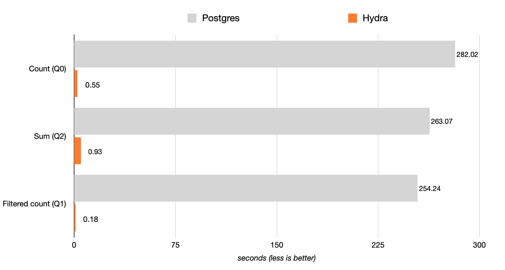
Query 0 is 512X faster:
SELECT COUNT(*) FROM hits;
Query 2 is 283X faster:
SELECT SUM(AdvEngineID), COUNT(*), AVG(ResolutionWidth) FROM hits;
Postgres COUNTs are slow? Not anymore! Hydra Columnar parallelizes and vectorizes aggregates (COUNT, SUM, AVG) to deliver the analytic speed you’ve always wanted on Postgres.
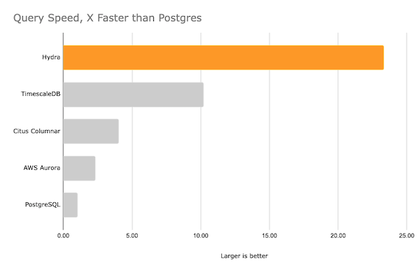
Filtering (WHERE clauses):
Query 1 is 1,412X faster:
SELECT COUNT(*) FROM hits WHERE AdvEngineID <> 0;
Filters on Hydra’s columnar storage resulted in a 1,412X performance improvement.
Review Clickbench for comprehensive results and the list of 42 queries tested.
This benchmark represents typical workload in the following areas: clickstream and traffic analysis, web analytics, machine-generated data, structured logs, and events data.
Figure F.2. Query Speed
For other continuous benchmark results, see BENCHMARKS.
F.21.6.2.1. Tables with large numbers of columns where only some columns are accessed #
When you have a large number of columns on your table (for example, a denormalized table) and need quick access to a subset of columns, Hydra Columnar can provide very fast access to just those columns without reading every column into memory.
F.21.7. Row vs Column Tables #
F.21.7.1. Columnar intro #
Columnar storage is a key part of the data warehouse, but why is that? In this article we will review what columnar storage is and why it’s such a key part of the data warehouse.
F.21.7.1.1. The heap table #
In traditional Postgres, data in Postgres is stored in a heap table. Heap tables are arranged row-by-row, similar to how you would arrange data when creating a large spreadsheet. Data can be added forever by appending data to the end of the table.
In Postgres, heap tables are organized into pages. Each page holds 8kb of data. Each page holds pointers to the start of each row in the data.
For more information, see Structure of a Heap Table, from The Internals of PostgreSQL.
Advantages
Heap tables are optimized for transactional queries. Heap tables can use indexes to quickly find the row of data you are looking for — an index holds the page and row number for particular values of data. Generally, transactional workloads will read, insert, update, or delete small amounts of data at a time. Performance can scale so long as you have indexes to find the data you’re looking for.
Shortcomings
Heap tables perform poorly when data cannot be found by an index, known as a table scan. In order to find the data, all data in the table must be read. Because the data is organized by row, you must read each row to find it. When you active dataset size grows beyond the available memory on the system, you will find these queries slow down tremendously.
Additionally, scans assisted by an index can only go so far if you are requesting a large amount of data. For example, if you would like to know the average over a given month and have an index on the timestamp, the index will help Postgres find the relevant data, but it will still need to read every target row individually in the table to compute the average.
F.21.7.1.2. Enter Columnar #
Columnar tables are organized transversely from row tables. Instead of rows being added one after another, rows are inserted in bulk into a stripe. Within each stripe, data from each column is stored next to each other. Imagine rows of a table containing:
| a | b | c | d |
| a | b | c | d |
| a | b | c | d |
This data would be stored as follows in columnar:
| a | a | a |
| b | b | b |
| c | c | c |
| d | d | d |
In columnar, you can think of each stripe as a row of metadata that also holds up to 150,000 rows of data. Within each stripe, data is divided into chunks of 10,000 rows, and then within each chunk, there is a “row” for each column of data you stored in it. Additionally, columnar stores the minimum, maximum, and count for each column in each chunk.
Advantages
Columnar is optimized for table scans — in fact, it doesn’t use indexes at all. Using columnar, it’s much quicker to obtain all data for a particular column. The database does not need to read data that you are not interested in. It also uses the metadata about the values in the chunks to eliminate reading data. This is a form of “auto-indexing” the data.
Because similar data is stored next to each other, very high data compression is possible. Data compression is an important benefit because columnar is often used to store huge amounts of data. By compressing the data, you can effectively read data more quickly from disk, which both reduces I/O and increasing effective fetch speed. It also has the effect of making better use of disk caching as data is cached in its compressed form. Lastly, you greatly reduce your storage costs.
Shortcomings
Hydra Columnar storage is not designed to do common transactional queries like “find by ID” - the database will need to scan a much larger amount of data to fetch this information than a row table.
Hydra Columnar is append-only. While it supports updates and deletes (also known as Data Modification Language or DML), space is not reclaimed on deletion, and updates insert new data. Updates and deletes lock the table as Columnar does not have a row-level construct that can be locked. Overall, DML is considerably slower on columnar tables than row tables. Space can be later reclaimed using columnar.vacuum.
Lastly, columnar tables need to be inserted in bulk in order
to create efficient stripes. This makes them ideal for
long-term storage of data you already have, but not ideal when
data is still streaming into the database. For these reasons,
it’s best to store data in row-based tables until it is ready
to be archived into columnar. You can compact small stripes by
calling
VACUUM.
F.21.7.2. Recommended Schema #
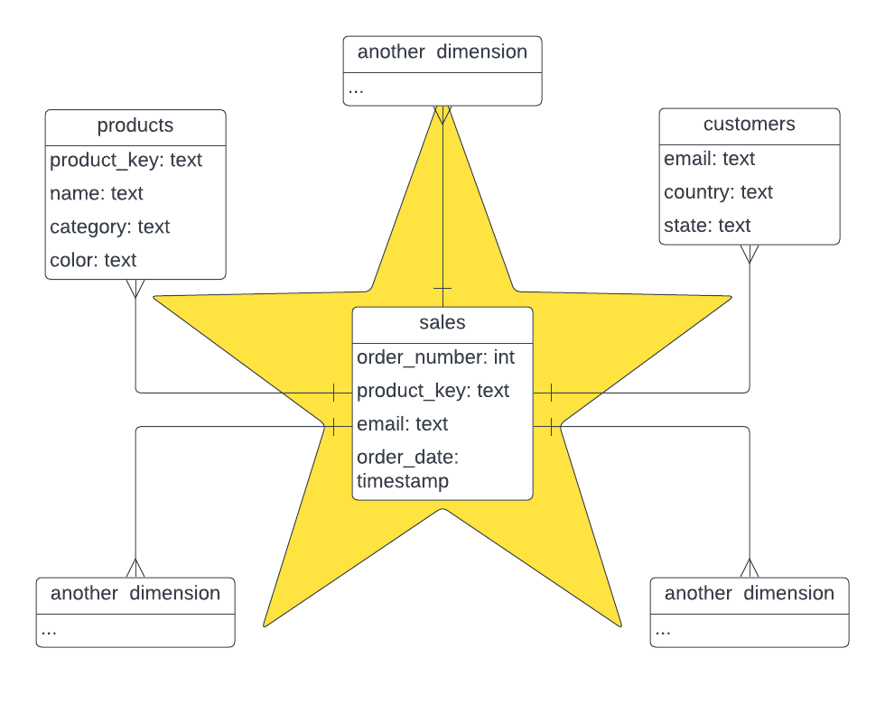
F.21.7.2.1. Star Schema #
Star schema is a logical arrangement of tables in a multidimensional database such that the entity relationship diagram resembles a star shape. It is a fundamental approach that is widely used to develop or build a data warehouse. It requires classifying model tables as either dimension or fact.
Fact tables record measurements or metrics for a specific event. A fact table contains dimension key columns that relate to dimension tables and numeric measure columns. Dimension tables describe business entities - the things you model. Entities can include products, people, places, and concepts including time itself. A dimension table contains a key column (or columns) that acts as a unique identifier and other descriptive columns. Fact tables are best as columnar tables, while dimension tables may be best as row tables due to their size and rate of updates.
The following diagram shows the star schema that we are going to model for the tutorial:
Figure F.3. star-schema
F.21.7.2.2. Hydra Columnar Schema #
A Hydra Columnar schema is conceptually identical to star schema with Fact tables record measurements / metics and Dimension tables are the entities that are modeled, such as people and places. The key difference of the Hydra Columnar schema is dimension tables may or may not be local within the Hydra Columnar database and can exist as foreign tables. Hydra Columnar schemas allow for rapidly updated data sets to avoid data duplication in the warehouse, but available for analysis instantly. To optimize for performance, foreign dimension tables should be kept under 1 million rows (though this varies by use case and data source). Larger tables should be imported and synced into Hydra Columnar.
F.21.8. Updates and Deletes #
Hydra Columnar tables support updates and deletes, yet remains an
append-only datastore. In order to achieve this, Hydra Columnar maintains
metadata about which rows in the table have been deleted or
modified. Modified data is re-written to the end of the table; you
can think of an UPDATE as a
DELETE followed by an
INSERT.
When querying, Hydra Columnar will automatically return only the latest version of your data.
F.21.8.1. Read Performance #
To maximize performance of SELECT queries,
columnar tables should have a maximum of data in every stripe.
Like an INSERT, each transaction with an
UPDATE query will write a new stripe. To
maximize the size of these stripes, update as much data in a
single transaction as possible. Alternatively, you can run
VACUUM on the table which will combine the
most recent stripes into a combined stripe of maximum size.
F.21.8.2. Write Performance #
Each updates or deletes query will lock the table, meaning
multiple UPDATE or DELETE
queries on the same table will be executed serially (one at a
time). UPDATE queries rewrite any rows that
are modified, and thus are relatively slow.
DELETE queries only modify metadata and thus
complete quite quickly.
F.21.8.3. Space Reclamation via VACUUM #
The columnar store provides multiple methods to vacuum and clean
up tables. Among these are the standard
VACUUM and VACUUM FULL
functionality, but also provided are UDFs, or User Defined
Functions that help for incremental vacuuming of large tables or
tables with many holes.
F.21.8.3.1. UDFs #
Vacuuming requires an exclusive lock while the data that is part of the table is reorganized and consolidated. This can cause other queries to pause until the vacuum is complete, thus stalling other activity in the database.
Using the vacuum UDF, you can specify the number of
stripes to consolidate in order to lower
the amount of time where a table is locked.
SELECT columnar.vacuum('mytable', 25);
Using the optional stripe count argument, a vacuum can be
performed incrementally. A value will return of how many
stripes were modified. Calling this function repeatedly is
fine, and it will continue to vacuum the table until there is
nothing more to do, and will return 0 as
the count.
| Parameter | Description | Default |
|---|---|---|
| table | Table name to vacuum | none, required |
| stripe_count | Number of stripes to vacuum |
0, or all
|
F.21.8.3.2. Vacuuming All #
In addition, you are provided a convenience function that can vacuum a whole schema, pausing between each vacuum and table to unlock and allow for other queries to continue on the database.
SELECT columnar.vacuum_full();
By default, this will vacuum the public
schema, but there are other options to control the vacuuming
process.
| Parameter | Description | Default |
|---|---|---|
| schema | Which schema to vacuum, if you have more than one schema, multiple calls will need to be made |
public
|
| sleep_time | The amount of time to sleep, in seconds, between vacuum calls |
0.1
|
| stripe_count | Number of stripes to vacuum per table between calls |
25
|
F.21.8.3.2.1. Examples #
SELECT columnar.vacuum_full('public');
SELECT columnar.vacuum_full(sleep_time => 0.5);
SELECT columnar.vacuum_full(stripe_count => 1000);
F.21.8.4. Isolation #
For terms used in this section, please refer to Section 13.2.
Hydra Columnar updates and deletes will meet the isolation level
requested for your current transaction (the default is
READ COMMITTED). Keep in mind that an
UPDATE query is implemented as a
DELETE followed by an
INSERT. As new data that is inserted in one
transaction can appear in a second transaction in
READ COMMITTED, this can affect concurrent
transactions even if the first transaction was an
UPDATE. While this satisfies
READ COMMITTED, it may result in unexpected
behavior. This is also possible in heap (row-based) tables, but
heap tables contain additional metadata that limit the impact of
this case.
For stronger isolation guarantees,
REPEATABLE READ is recommended. In this
isolation level, your transaction will be cancelled if it
references data that has been modified by another transaction.
In this case, your application should be prepared to retry the
transaction.
F.21.9. Optimizing Query Performance #
F.21.9.1. Column Cache #
The columnar store makes extensive use of compression, allowing for your data to be stored efficiently on disk and in memory as compressed data.
While this is very helpful, in some circumstances a long running analytical query can retrieve and decompress the same columns on a recurring basis. In order to counter that, a column caching mechanism is available to store uncompressed data in-memory, up to a specified amount of memory per worker.
These uncompressed columns are then available for the lifetime
of a SELECT query, and are managed by the
columnar store directly. NOTE that this cache is not used for
UPDATE, DELETE, or
INSERT, and are released after the
SELECT query is complete. #### Enabling the
Cache
Caching is be enabled or disabled with a GUC:
columnar.enable_column_cache. For queries where the cache is not helpful, you may find
slightly better performance by disabling the cache.
-- enable the cache
set columnar.enable_column_cache = 't';

-- disable the cache
set columnar.enable_column_cache = 'f';
In addition, the cache size can be set, with a default of
200MB per process.
set columnar.column_cache_size = '2000MB';
This size can range between 20MB and
20000MB, and is consumed by each parallel
process. This means that if you have 8
parallel processes and set the cache size to
2000MB, then a query can consume up to
8 * 2000000 bytes, or up to
16GB of RAM, so it is very important to
choose a cache size that is appropriate for your workload.
F.21.9.2. Vacuum Tables #
Vacuuming tables will optimize tables that have had many inserts, updates, or deletes. There are three levels of vacuum on columnar tables:
VACUUM tablewill rewrite recently created stripes into optimal stripes of maximum size. If making many small inserts or updates into a columnar table, runVACUUMfrequently to optimize the table.SELECT columnar.vacuum_all()will reclaim space from updated and deleted rows, writing new optimal stripes and compact the amount of space the table occupies.VACUUM FULL tablewill do a full rewrite of the table making fully optimized stripes. This operation is very expensive but produces the best results.
F.21.10. Materialized Views #
Unlike regular views, which are virtual tables that run a query each time they are accessed, materialized views are precomputed database tables that store the results of a query and only update them when they are directly refreshed. Compared to performing equivalent queries on the underlying tables, materialized views can significantly enhance the speed of your queries, particularly for more complex queries.
Materialized views are typically used in scenarios where query performance is critical, queries are executed frequently against large and complex data sets, and the data being queried doesn’t change as frequently. In cases where your queried data requires multiple aggregations, joins, and operations that are computed frequently for reporting or analytics, you can efficiently improve performance and reduce execution time using precomputed materialized views.
You can create a materialized view using the following command:
CREATE MATERIALIZED VIEW [ IF NOT EXISTS ] view_name
    [ (column_name [, ...] ) ]
    [ USING method ]
    AS query
    [ WITH [ NO ] DATA ]
You can set
USING columnarto store large materialized views in columnar for fast analyticsYou can set
USING heapfor traditional row-based materialized views
For example, here’s a materialized view that computes a monthly sales summary containing the total products sold and sales gained:
CREATE MATERIALIZED VIEW sales_summary
  USING columnar
AS
SELECT
    date_trunc('month', order_date) AS month,
    product_id,
    SUM(quantity) AS total_quantity,
    SUM(quantity * price) AS total_sales
FROM
    sales
GROUP BY
    date_trunc('month', order_date),
    product_id;
You can refresh your materialized view with the latest data using
REFRESH MATERIALIZED VIEW [ CONCURRENTLY ] view_name.
Using the CONCURRENTLY option will allow the
view to be refreshed while allowing queries to continue on the
current data, but requires a unique index on the view.
F.21.10.1. Best Practices for Materialized Views #
There are a couple of things you can do to make sure you’re making the most of materialized views:
Refresh your materialized view: The frequency and methods you employ to refresh your materialized view are crucial factors that influence the overall effectiveness of your view. As refreshing a materialized view can be a resource-intensive operation, it’s better suited to data that updates infrequently.
Monitor disk space and performance: Materialized views can consume significant amounts of disk space, so it’s essential to monitor their size and delete unused ones to free up space. You should also monitor their refresh performance to ensure that they don’t negatively impact the overall performance.
Add indexes to optimize your queries: Materialized views offer a distinct advantage by being stored as regular tables in Postgres. This means that they can fully leverage the benefits of indexing techniques, leading to enhanced performance and efficient processing of large data sets.
F.21.10.2. Incremental Materialized Views with pg_ivm #
Documentation in this section is courtesy
pg_ivm.
pg_ivm provides a way to make materialized
views up-to-date where only incremental changes are computed and
applied on views rather than recomputing the contents from
scratch as REFRESH MATERIALIZED VIEW does.
This process is called “incremental view maintenance” (or IVM),
and it can update materialized views more efficiently than
recomputation when only small parts of the view are changed.
There are two approaches with regard to timing of view
maintenance: immediate and deferred. In immediate maintenance,
views are updated in the same transaction that its base table is
modified. In deferred maintenance, views are updated after the
transaction is committed, for example, when the view is
accessed, as a response to user command like
REFRESH MATERIALIZED VIEW, or periodically in
background, and so on. pg_ivm provides a kind
of immediate maintenance, in which materialized views are
updated immediately in AFTER triggers when a base table is
modified.
To begin using pg_ivm, you must first enable
it on your database:
CREATE EXTENSION IF NOT EXISTS pg_ivm;
We call a materialized view supporting IVM an Incrementally
Maintainable Materialized View (IMMV). To create an IMMV, you
have to call create_immv function with a
relation name and a view definition query. For example:
SELECT create_immv('sales_test', 'SELECT * FROM sales');
creates an IMMV with name ‘sales_test’ defined as
SELECT * FROM sales. This corresponds to the
following command to create a normal materialized view:
CREATE MATERIALIZED VIEW sales_test AS SELECT * FROM sales;
When an IMMV is created, some triggers are automatically created so that the view’s contents are immediately updated when its base tables are modified.
postgres=# SELECT create_immv('m', 'SELECT * FROM t0');
NOTICE:  could not create an index on immv "m" automatically
DETAIL:  This target list does not have all the primary key columns, or this view does not contain DISTINCT clause.
HINT:  Create an index on the immv for efficient incremental maintenance.
 create_immv
-------------
           3
(1 row)

postgres=# SELECT * FROM m;
 i
---
 1
 2
 3
(3 rows)

postgres=# INSERT INTO t0 VALUES (4);
INSERT 0 1
postgres=# SELECT * FROM m; -- automatically updated
 i
---
 1
 2
 3
 4
(4 rows)
F.21.10.2.1. IMMV and Columnar #
You can create an IMMV using columnar store by setting the default table access method. If the source table is columnar, you must also disable parallelism temporarily to create the IMMV:
SET default_table_access_method = 'columnar';
SET max_parallel_workers = 1;
SELECT create_immv('sales_test', 'SELECT * FROM sales');
After the IMMV is created, you can restore the settings to their defaults. (These settings do not affect other connections and will also be restored to their defaults upon your next session.)
SET max_parallel_workers = DEFAULT;
SET default_table_access_method = DEFAULT;
F.21.10.2.2. Functions #
F.21.10.2.2.1. create_immv #
Use create_immv function to create IMMV.
create_immv(immv_name text, view_definition text) RETURNS bigint
create_immv defines a new IMMV of a
query. A table of the name immv_name is
created and a query specified by
view_definition is executed and used to
populate the IMMV. The query is stored in
pg_ivm_immv, so that it can be refreshed
later upon incremental view maintenance.
create_immv returns the number of rows in
the created IMMV.
When an IMMV is created, triggers are automatically created so that the view’s contents are immediately updated when its base tables are modified. In addition, a unique index is created on the IMMV automatically if possible. If the view definition query has a GROUP BY clause, a unique index is created on the columns of GROUP BY expressions. Also, if the view has DISTINCT clause, a unique index is created on all columns in the target list. Otherwise, if the IMMV contains all primary key attributes of its base tables in the target list, a unique index is created on these attributes. In other cases, no index is created.
F.21.10.2.2.2. refresh_immv #
Use refresh_immv function to refresh
IMMV.
refresh_immv(immv_name text, with_data bool) RETURNS bigint
refresh_immv completely replaces the
contents of an IMMV as
REFRESH MATERIALIZED VIEW command does
for a materialized view. To execute this function you must
be the owner of the IMMV. The old contents are discarded.
The with_data flag is corresponding to
WITH [NO] DATA option of
REFRESH MATERIALIZED VIEW command. If
with_data is true, the backing query is executed to provide
the new data, and if the IMMV is unpopulated, triggers for
maintaining the view are created. Also, a unique index is
created for IMMV if it is possible and the view doesn’t have
that yet. If with_data is false, no new data is generated
and the IMMV become unpopulated, and the triggers are
dropped from the IMMV. Note that unpopulated IMMV is still
scannable although the result is empty. This behaviour may
be changed in future to raise an error when an unpopulated
IMMV is scanned.
F.21.10.2.2.3. get_immv_def #
get_immv_def reconstructs the underlying
SELECT command for an IMMV. (This is a decompiled
reconstruction, not the original text of the command.)
get_immv_def(immv regclass) RETURNS text
F.21.10.2.2.4. IMMV metadata catalog #
The catalog pg_ivm_immv stores IMMV
information.
| Name | Type | Description |
|---|---|---|
| immvrelid | regclass | The OID of the IMMV |
| viewdef | text | Query tree (in the form of a nodeToString() representation) for the view definition |
| ispopulated | bool | True if IMMV is currently populated |
F.21.10.2.3. Example #
In general, IMMVs allow faster updates than
REFRESH MATERIALIZED VIEW at the price of
slower updates to their base tables. Update of base tables is
slower because triggers will be invoked and the IMMV is
updated in triggers per modification statement.
For example, suppose a normal materialized view defined as below:
test=# CREATE MATERIALIZED VIEW mv_normal AS
        SELECT a.aid, b.bid, a.abalance, b.bbalance
        FROM pgbench_accounts a JOIN pgbench_branches b USING(bid);
SELECT 10000000
Updating a tuple in a base table of this materialized view is
rapid but the REFRESH MATERIALIZED VIEW
command on this view takes a long time:
test=# UPDATE pgbench_accounts SET abalance = 1000 WHERE aid = 1;
UPDATE 1
Time: 9.052 ms

test=# REFRESH MATERIALIZED VIEW mv_normal ;
REFRESH MATERIALIZED VIEW
Time: 20575.721 ms (00:20.576)
On the other hand, after creating IMMV with the same view definition as below:
test=# SELECT create_immv('immv',
        'SELECT a.aid, b.bid, a.abalance, b.bbalance
         FROM pgbench_accounts a JOIN pgbench_branches b USING(bid)');
NOTICE:  created index "immv_index" on immv "immv"
 create_immv
-------------
    10000000
(1 row)
updating a tuple in a base table takes more than the normal
view, but its content is updated automatically and this is
faster than the REFRESH MATERIALIZED VIEW
command.
test=# UPDATE pgbench_accounts SET abalance = 1234 WHERE aid = 1;
UPDATE 1
Time: 15.448 ms

test=# SELECT * FROM immv WHERE aid = 1;
 aid | bid | abalance | bbalance
-----+-----+----------+----------
   1 |   1 |     1234 |        0
(1 row)
An appropriate index on IMMV is necessary for efficient IVM because we need to looks for tuples to be updated in IMMV. If there are no indexes, it will take a long time.
Therefore, when an IMMV is created by the
create_immv function, a unique index is
created on it automatically if possible. If the view
definition query has a GROUP BY clause, a unique index is
created on the columns of GROUP BY expressions. Also, if the
view has DISTINCT clause, a unique index is created on all
columns in the target list. Otherwise, if the IMMV contains
all primary key attributes of its base tables in the target
list, a unique index is created on these attributes. In other
cases, no index is created.
In the previous example, a unique index “immv_index” is created on aid and bid columns of “immv”, and this enables the rapid update of the view. Dropping this index make updating the view take a loger time.
test=# DROP INDEX immv_index;
DROP INDEX

test=# UPDATE pgbench_accounts SET abalance = 9876 WHERE aid = 1;
UPDATE 1
Time: 3224.741 ms (00:03.225)
F.21.10.2.4. Supported View Definitions and Restriction #
Currently, IMMV’s view definition can contain inner joins,
DISTINCT clause, some built-in aggregate functions, simple
sub-queries in FROM clause, and simple CTE
(WITH query). Inner joins including
self-join are supported, but outer joins are not supported.
Supported aggregate functions are count, sum, avg, min and
max. Other aggregates, sub-queries which contain an aggregate
or DISTINCT clause, sub-queries in other
than FROM clause, window functions,
HAVING, ORDER BY,
LIMIT/OFFSET,
UNION/INTERSECT/EXCEPT,
DISTINCT ON,
TABLESAMPLE, VALUES, and
FOR UPDATE/SHARE can not
be used in view definition.
The base tables must be simple tables. Views, materialized views, inheritance parent tables, partitioned tables, partitions, and foreign tables can not be used.
The targetlist cannot contain system columns, columns whose
name starts with __ivm_.
Logical replication is not supported, that is, even when a base table at a publisher node is modified, IMMVs at subscriber nodes defined on these base tables are not updated.
F.21.10.2.5. Limitations and Restrictions #
F.21.10.2.5.1. Aggregates #
Supported aggregate functions are count,
sum, avg,
min, and max.
Currently, only built-in aggregate functions are supported
and user defined aggregates cannot be used.
When an IMMV including aggregate is created, some extra
columns whose name start with __ivm are
automatically added to the target list.
__ivm_count__ contains the number of
tuples aggregated in each group. In addition, more than one
extra columns for each column of aggregated value are added
in order to maintain the value. For example, columns named
like __ivm_count_avg__ and
__ivm_sum_avg__ are added for maintaining
an average value. When a base table is modified, the new
aggregated values are incrementally calculated using the old
aggregated values and values of related extra columns stored
in the IMMV.
Note that for min or
max, the new values could be
re-calculated from base tables with regard to the affected
groups when a tuple containing the current minimal or
maximal values are deleted from a base table. Therefore, it
can takes a long time to update an IMMV containing these
functions.
Also, note that using sum or
avg on real
(float4) type or
double precision
(float8) type in IMMV is unsafe, because
aggregated values in IMMV can become different from results
calculated from base tables due to the limited precision of
these types. To avoid this problem, use the
numeric type instead.
F.21.10.2.5.2. Restrictions on Aggregate #
If we have a GROUP BY clause, expressions
specified in GROUP BY must appear in the
target list. This is how tuples to be updated in the IMMV
are identified. These attributes are used as scan keys for
searching tuples in the IMMV, so indexes on them are
required for efficient IVM.
Targetlist cannot contain expressions which contain an aggregate in it.
F.21.10.2.5.3. Subqueries #
Simple subqueries in FROM clause are
supported.
F.21.10.2.5.4. Restrictions on Subqueries #
Subqueries can be used only in FROM
clause. Subqueries in target list or
WHERE clause are not supported.
Subqueries containing an aggregate function or
DISTINCT are not supported.
F.21.10.2.6. CTE #
Simple CTEs (WITH queries) are supported.
F.21.10.2.6.1. Restrictions on CTEs #
WITH queries containing an aggregate
function or DISTINCT are not supported.
Recursive queries (WITH RECURSIVE) are
not allowed. Unreferenced CTEs are not allowed either, that
is, a CTE must be referenced at least once in the view
definition query.
F.21.10.2.6.2. DISTINCT #
DISTINCT is allowed in IMMV’s definition
queries. Suppose an IMMV defined with DISTINCT on a base
table containing duplicate tuples. When tuples are deleted
from the base table, a tuple in the view is deleted if and
only if the multiplicity of the tuple becomes zero.
Moreover, when tuples are inserted into the base table, a
tuple is inserted into the view only if the same tuple
doesn’t already exist in it.
Physically, an IMMV defined with DISTINCT
contains tuples after eliminating duplicates, and the
multiplicity of each tuple is stored in a extra column named
__ivm_count__ that is added when such
IMMV is created.
F.21.10.2.6.3. TRUNCATE #
When a base table is truncated, the IMMV is also truncated
and the contents become empty if the view definition query
does not contain an aggregate without a
GROUP BY clause. Aggregate views without
a GROUP BY clause always have one row.
Therefore, in such cases, if a base table is truncated, the
IMMV is simply refreshed instead of being truncated.
F.21.10.2.6.4. Concurrent Transactions #
Suppose an IMMV is defined on two base tables and each table
was modified in different a concurrent transaction
simultaneously. In the transaction which was committed
first, the IMMV can be updated considering only the change
which happened in this transaction. On the other hand, in
order to update the IMMV correctly in the transaction which
was committed later, we need to know the changes occurred in
both transactions. For this reason,
ExclusiveLock is held on an IMMV
immediately after a base table is modified in
READ COMMITTED mode to make sure that the
IMMV is updated in the latter transaction after the former
transaction is committed. In
REPEATABLE READ or
SERIALIZABLE mode, an error is raised
immediately if lock acquisition fails because any changes
which occurred in other transactions are not be visible in
these modes and IMMV cannot be updated correctly in such
situations. However, as an exception if the IMMV has only
one base table and doesn’t use DISTINCT or GROUP BY, and the
table is modified by INSERT, then the
lock held on the IMMV is
RowExclusiveLock.
F.21.10.2.6.5. Row Level Security #
If some base tables have row level security policy, rows that are not visible to the materialized view’s owner are excluded from the result. In addition, such rows are excluded as well when views are incrementally maintained. However, if a new policy is defined or policies are changed after the materialized view was created, the new policy will not be applied to the view contents. To apply the new policy, you need to recreate IMMV.
F.21.10.2.6.6. How to Disable or Enable Immediate Maintenance #
IVM is effective when we want to keep an IMMV up-to-date and small fraction of a base table is modified infrequently. Due to the overhead of immediate maintenance, IVM is not effective when a base table is modified frequently. Also, when a large part of a base table is modified or large data is inserted into a base table, IVM is not effective and the cost of maintenance can be larger than refresh from scratch.
In such situation, we can use refesh_immv
function with with_data = false to
disable immediate maintenance before modifying a base table.
After a base table modification, call
refresh_immvwith
with_data = true to refresh the view data
and enable immediate maintenance.
F.21.11. Vectorized Execution #
Vectorized execution is a technique that is used to improve the performance of database queries by executing multiple operations simultaneously. This is in contrast to traditional execution, where each operation is performed one at a time.
Vectorized execution works by dividing data into small chunks, called vectors, and then executing multiple operations on each vector in parallel. This allows the database to take advantage of modern processors, which are designed to perform multiple operations simultaneously, and can significantly improve the performance of queries that involve large amounts of data.
For example, consider a query that calculates the sum of a column of numbers in a table. In traditional execution, the database would go through each row of the table one at a time, adding each number to the running total. With vectorized execution, the database would divide the data into vectors, and then use multiple processor cores to add the numbers in each vector simultaneously. This can significantly reduce the time it takes to perform the query.
By taking advantage of modern processors and executing multiple operations simultaneously, vectorized execution can significantly improve the speed and efficiency of database queries.
F.21.12. Query Parallelization #
Query parallelization is a technique that is used to improve the performance of database queries by executing them in parallel across multiple processor cores or machines. This is in contrast to traditional serial execution, where each operation is performed one at a time.
Query parallelization works by dividing the work of a query into smaller tasks, which are then executed simultaneously on multiple cores or machines. This allows the database to take advantage of modern processors, which are designed to perform multiple operations simultaneously, and can significantly improve the performance of queries that involve large amounts of data.
For example, consider a query that calculates the sum of a column of numbers in a table. In traditional serial execution, the database would go through each row of the table one at a time, adding each number to the running total. With query parallelization, the database would divide the data into smaller chunks and distribute them among multiple cores or machines, which would then calculate the sum of their respective chunks simultaneously. This can significantly reduce the time it takes to perform the query.
By taking advantage of modern processors and executing queries in parallel, query parallelization can significantly improve the speed and efficiency of database operations.
F.21.13. Common recomendations #
F.21.13.1. Choosing Stripe Size and Chunk Size #
Determining the optimal stripe and chunk sizes for columnar tables
in Tantor SE depends on
various factors, such as the nature of the data, query patterns, and hardware characteristics.
Here are some recommendations:
Stripe Size: The optimal stripe size may depend on the typical size of your queries. If queries usually return a large number of rows, a larger stripe size might be more efficient, as it reduces the number of input/output operations. On the other hand, if queries often return a small subset of data, a smaller stripe size might be preferable.
Chunk Size: This determines how much data will be compressed at a time. A smaller chunk size might lead to a higher compression ratio, but can increase the overhead of compression. A larger chunk size can reduce overhead, but potentially decrease the compression ratio.
Testing and Tuning: It is important to conduct testing with real data and queries to determine the optimal settings for your specific situation. You can start with the default recommended settings, and then experiment with different stripe and chunk sizes to see how it affects query performance and compression ratios.
Hardware Properties: It's also worth considering the characteristics of your hardware, such as disk and CPU throughput, as this can influence which stripe and chunk sizes are most effective.
Ultimately, the optimal stripe and chunk sizes depend on the unique characteristics of your environment, data, and query patterns.
F.21.13.2. Compression Algorithms #
The choice of compression algorithm for columnar tables in Tantor SE
depends on several factors, including the nature of the data, performance requirements,
and hardware specifications. Here are some recommendations that may help you make a decision:
none: This type applies no compression to the data. It can be useful if your data is already compressed, or if you have very high performance requirements and sufficient disk space.lz4: provides fast data compression and decompression. This can be useful if you have high performance requirements, but still want to save some disk space.zstd: offers a higher compression ratio compared toLZ4, but requires more CPU time for compressing and decompressing data. This algorithm can be beneficial if you have limited disk space and are willing to spend a bit more CPU time on data compression.
It is important to note that choosing a compression algorithm is a trade-off between performance (compression and decompression speed) and disk space. Also, the efficiency of each compression algorithm can greatly depend on the nature of your data. Therefore, it is recommended to conduct some tests with your real data and queries to determine the most suitable compression algorithm for your situation.
F.21.14. Working with Time Series Data #
F.21.14.1. Creating Tables #
Time Series data is characterized by the sequential recording of values in increasing time order. For such data, orderliness is important.
Create the necessary extensions:
create extension pg_columnar;
create extension plpython3u;
Create a test table:
CREATE TABLE perf_columnar(
    id INT8,
    ts TIMESTAMPTZ,
    customer_id INT8,
    vendor_id INT8,
    name TEXT,
    description TEXT,
    value NUMERIC,
    quantity INT4
) USING columnar;

SELECT columnar.alter_columnar_table_set(
    'public.perf_columnar',
    compression => 'lz4',
    stripe_row_limit => 100000,
    chunk_group_row_limit => 10000
);
Create a function to generate random text:
CREATE OR REPLACE FUNCTION random_words(n INT4) RETURNS TEXT LANGUAGE plpython3u AS $$
import random
t = ''
words = ['zero','one','two','three','four','five','six','seven','eight','nine','ten']
for i in range(0, n):
  if (i != 0):
    t += ' '
  r = random.randint(0, len(words) - 1)
  t += words[r]
return t
$$;
Generate test data:
INSERT INTO perf_columnar
   SELECT
    g, -- id
    '2023-06-01'::timestamptz + ('1 minute'::interval * g), -- ts
    (random() * 1000000)::INT4, -- customer_id
    (random() * 100)::INT4, -- vendor_id
    random_words(7), -- name
    random_words(100), -- description
    (random() * 100000)::INT4/100.0, -- value
    (random() * 100)::INT4 -- quantity
   FROM generate_series(1,7500000) g;
As seen from the query above, we have inserted data sorted by ts.
Gather statistics using VACUUM (ANALYZE, VERBOSE):
VACUUM ANALYZE perf_columnar;
Create a copy of the table with different parameters:
CREATE TABLE perf_columnar2(LIKE perf_columnar) USING COLUMNAR;

SELECT columnar.alter_columnar_table_set(
    'public.perf_columnar2',
    compression => 'zstd',
    stripe_row_limit => 10000,
    chunk_group_row_limit => 1000
);

INSERT INTO perf_columnar2 SELECT * FROM perf_columnar;

VACUUM ANALYZE perf_columnar2;
Check the size of the resulting tables:
test_db=# \dt+
                                        List of relations
 Schema |      Name      | Type  |  Owner   | Persistence | Access method |  Size   | Description
--------+----------------+-------+----------+-------------+---------------+---------+-------------
 public | perf_columnar  | table | postgres | permanent   | columnar      | 1886 MB |
 public | perf_columnar2 | table | postgres | permanent   | columnar      | 850 MB  |
(2 rows)
As can be seen, the table perf_columnar is twice as large as perf_columnar2.
Check the options of the tables:
test_db=# select * from columnar.options;

    relation    | chunk_group_row_limit | stripe_row_limit | compression | compression_level
----------------+-----------------------+------------------+-------------+-------------------
 perf_columnar  |                 10000 |           100000 | lz4         |                 3
 perf_columnar2 |                  1000 |            10000 | zstd        |                 3

(2 rows)
F.21.14.2. Comparing Query Performance #
Execute a typical query to read a set of records from the perf_columnar table
for a specific time interval:
explain (analyze, verbose, buffers) select ts from perf_columnar
where ts < '2023-06-01 10:00:00'::timestamp with time zone and
      ts > '2023-06-01 10:00:05'::timestamp with time zone;
                                                                           QUERY PLAN
-----------------------------------------------------------------------------------------------------------------------------------------------------------------
 Custom Scan (ColumnarScan) on public.perf_columnar  (cost=0.00..401.12 rows=4 width=8) (actual time=18.838..49.001 rows=4 loops=1)
   Output: ts
   Filter: ((perf_columnar.ts < '2023-06-01 10:00:00+03'::timestamp with time zone) AND (perf_columnar.ts > '2023-06-01 10:00:05+03'::timestamp with time zone))
   Rows Removed by Filter: 9996
   Columnar Projected Columns: ts
   Columnar Chunk Group Filters: ((ts < '2023-06-01 10:00:00+03'::timestamp with time zone) AND (ts > '2023-06-01 10:00:05+03'::timestamp with time zone))
   Columnar Chunk Groups Removed by Filter: 749     <-----------
   Buffers: shared hit=3833 read=264                <-----------
 Query Identifier: 1607994334608619710
 Planning:
   Buffers: shared hit=52 read=7
 Planning Time: 12.789 ms
 Execution Time: 49.188 ms
(13 rows)
Execute a typical query to read a set of records from the perf_columnar2 table
for a specific time interval:
explain (analyze, verbose, buffers) select ts from perf_columnar2
where ts < '2020-01-01 10:00:00'::timestamp with time zone and
      ts > '2020-01-01 10:00:05'::timestamp with time zone;
                                                                            QUERY PLAN
-------------------------------------------------------------------------------------------------------------------------------------------------------------------
 Custom Scan (ColumnarScan) on public.perf_columnar2  (cost=0.00..17.95 rows=52 width=8) (actual time=5.175..58.532 rows=49 loops=1)
   Output: ts
   Filter: ((perf_columnar2.ts < '2020-01-01 10:00:00+03'::timestamp with time zone) AND (perf_columnar2.ts > '2020-01-01 10:00:05+03'::timestamp with time zone))
   Rows Removed by Filter: 951
   Columnar Projected Columns: ts
   Columnar Chunk Group Filters: ((ts < '2020-01-01 10:00:00+03'::timestamp with time zone) AND (ts > '2020-01-01 10:00:05+03'::timestamp with time zone))
   Columnar Chunk Groups Removed by Filter: 7499    <-----------
   Buffers: shared hit=40824 read=1                 <-----------
 Query Identifier: -801549076851693482
 Planning:
   Buffers: shared hit=155
 Planning Time: 1.086 ms
 Execution Time: 58.717 ms
(13 rows)
Note Columnar Chunk Groups Removed by Filter: 749 in the first case and 7499 in the second.
However, the number of read buffers in the second query is much higher.
Terminology for understanding the behavior of these queries:
Stripe: This type does not apply any compression to the data. It can be useful if your data is already compressed, or if you have very high performance requirements and sufficient disk space.Chunk Group: stripes are divided into chunk groups of 10,000 rows (by default).Chunk: Each chunk group consists of one chunk for each column.Chunkis the unit of compression, and min/max values are tracked for each chunk, enabling chunk group filtering (Chunk Group Filtering).Chunk Group Filtering: when a query'sWHEREclause does not match any tuples in the chunk, and we can determine this from the min/max value for the chunk, then chunk group filtering simply skips the whole chunk group without unpacking it.
As can be seen, 749/7499 chunk groups were filtered, meaning
that 7490000/7499000 rows were filtered without the need to extract or unpack
the data. Only 1 chunk group (10,000 and 1,000 rows) needed to be extracted and
unpacked, so the query took only milliseconds.
But as seen from the query plans, in the first case, 30 MB was used, while in the second, ten times more - 319 MB.
F.21.14.3. Using Indexes #
Columnar supports btree and hash indexes (and constraints that require them),
but does not support index types like gist, gin,
spgist, and brin.
Consider creating indexes for the tables perf_columnar and
perf_columnar2:
create index test on perf_columnar2 (ts);
create index test_h on perf_columnar (ts);
Check the size of the indexes:
test_db=# \di+
                                            List of relations

 Schema |  Name  | Type  |  Owner   |     Table      | Persistence | Access method |  Size  | Description
--------+--------+-------+----------+----------------+-------------+---------------+--------+-------------
 public | test   | index | postgres | perf_columnar2 | permanent   | btree         | 161 MB |
 public | test_h | index | postgres | perf_columnar  | permanent   | btree         | 161 MB |
(2 rows)
The sizes of the indexes are the same.
Disable the forced use of Custom Scan:
SET columnar.enable_custom_scan TO false;
Re-execute the typical query to read a set of records from the perf_columnar table
for a specific time interval:
explain (analyze, verbose, buffers) select ts from perf_columnar
where ts < '2023-06-01 10:00:00'::timestamp with time zone and
      ts > '2023-06-01 10:00:05'::timestamp with time zone;
                                                                             QUERY PLAN
---------------------------------------------------------------------------------------------------------------------------------------------------------------------
 Index Scan using test_h on public.perf_columnar  (cost=0.43..3217.48 rows=4 width=8) (actual time=402.144..402.204 rows=4 loops=1)
   Output: ts
   Index Cond: ((perf_columnar.ts < '2023-06-01 10:00:00+03'::timestamp with time zone) AND (perf_columnar.ts > '2023-06-01 10:00:05+03'::timestamp with time zone))
   Buffers: shared hit=181 read=3232      <-----------
 Query Identifier: 1607994334608619710
 Planning:
   Buffers: shared hit=20 read=5
 Planning Time: 16.278 ms
 Execution Time: 402.386 ms
(9 rows)
Nearly the same number of buffers were scanned as when using
Custom Scan.
Re-execute the typical query to read a set of records from the perf_columnar2 table
for a specific time interval:
explain (analyze, verbose, buffers) select ts from perf_columnar2
where ts < '2020-01-01 10:00:00'::timestamp with time zone and
      ts > '2020-01-01 10:00:05'::timestamp with time zone;
                                                                              QUERY PLAN
-----------------------------------------------------------------------------------------------------------------------------------------------------------------------
 Index Scan using test on public.perf_columnar2  (cost=0.43..153.05 rows=52 width=8) (actual time=14.620..14.821 rows=49 loops=1)
   Output: ts
   Index Cond: ((perf_columnar2.ts < '2020-01-01 10:00:00+03'::timestamp with time zone) AND (perf_columnar2.ts > '2020-01-01 10:00:05+03'::timestamp with time zone))
   Buffers: shared hit=372 read=145     <-----------
 Query Identifier: -801549076851693482
 Planning:
   Buffers: shared hit=97
 Planning Time: 0.813 ms
 Execution Time: 14.978 ms
(13 rows)
For the second table, far fewer buffers were scanned, and the query is executed in the most optimal manner.
F.21.14.4. Conclusions #
The following conclusions can be drawn:
The most effective data compression method is
zstd;The size of the stripe and chunk affects the amount of buffers scanned using the
Chunk Group Filteringmethod;When reading a small amount of data, using an index may prove to be more efficient;
To test the hypothesis, it is necessary to forcibly enable the use of indexes with the command
SET columnar.enable_custom_scan TO false;Sequential recording of TS data can significantly reduce the size of indexes and the volume of unpacked chunks (
Chunk). Therefore, it is recommended to sort data before inserting it into the database or use clustering (cluster).